Breast — Xenium transcriptomics + H&E histology¶

This tutorial runs LYNX on a triple-positive breast-cancer sample that pairs Xenium (the reference spatial transcriptomics modality) with H&E histology image patches (the query modality).
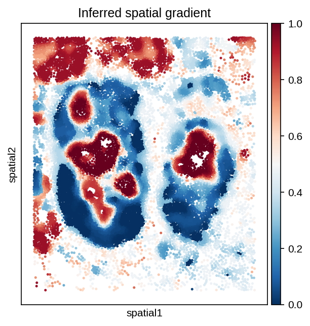
The spatial gradients from an immune-enriched region to two separate tumor states (DCIS, Invasive tumor) are best captured by a branching structure with distinct stromal environments, so here LYNX fits a principal tree (rather than a single curve) over the latent embedding.
We show the training pipeline as code, then load a pre-saved result snapshot for the downstream tree inference and plots. Pathway-signature analyses from the full study (stromal subtyping, single-gene / signature dynamics) are intentionally omitted to keep this minimal.

[ ]:

import os
import numpy as np
import scanpy as sc
import squidpy as sq
import scFates as scf
import torch
import torch.nn as nn

import matplotlib.pyplot as plt
from matplotlib import rcParams
rcParams.update({"figure.dpi": 120, "savefig.dpi": 300})
import lynx

/home/yinuo/Desktop/azizi_lab/IMS/env/lib/python3.9/site-packages/numba/core/decorators.py:282: RuntimeWarning: nopython is set for njit and is ignored
  warnings.warn('nopython is set for njit and is ignored', RuntimeWarning)

1. Load and filter the paired modalities¶

[2]:

# Dataset specs
n_subgraphs = 16
k = 8
r = 50
# Model / training parameters
n_hidden, n_latent = 32, 6
n_epochs, lr, patience = 500, 1e-3, 20

data_path = "../../data/breast/dcis_fov/"
adata_xenium = sc.read_h5ad(os.path.join(data_path, "cell_feature_matrix.h5"))  # Aligned Xenium data
adata_he = sc.read_h5ad(os.path.join(data_path, "he_patches_norm.h5ad")) # Aligned histology patches w.r.t. to each Xenium cell
cluster_key = "cell_type"

# Drop unlabeled / hybrid / extremely rare annotations (e.g. < 10 cells); unify labels.
rare_labels = adata_xenium.obs[cluster_key].value_counts()[
    adata_xenium.obs[cluster_key].value_counts() < 10
].index.to_list()
labeled_mask = np.logical_and(
    adata_xenium.obs[cluster_key] != "Unlabeled",
    ~adata_xenium.obs[cluster_key].isin(rare_labels),
)
hybrid_mask = adata_xenium.obs[cluster_key].str.contains("Hybrid", case=False)
labeled_mask = np.logical_and(labeled_mask, ~hybrid_mask)
adata_xenium.obs[cluster_key] = (
    adata_xenium.obs[cluster_key]
    .astype(str)
    .replace({"DCIS_1": "DCIS", "Prolif_Invasive_Tumor": "Invasive_Tumor"})
    .astype("category")
)

adata_xenium = adata_xenium[labeled_mask].copy()
adata_xenium.obs.index = adata_xenium.obs.index.astype(int)
adata_he = adata_he[labeled_mask].copy()
patch_size = np.sqrt(adata_he.var.shape[0] // 3).astype(int)  # H&E patch side length

2. Build the spatial hetero-graph, configure the model¶

[3]:

graph_data = lynx.dataset.HeteroDataset(
    adatas_ref=adata_xenium,
    adatas_query=adata_he,
    n_subgraphs=n_subgraphs,
    k=k, r=r,
    is_weighted=True,
    cluster_key=cluster_key,
    alpha=0.5,
    query="HE", query_proj_key="spatial",
    ref="Xenium", ref_proj_key="spatial",
)

train_configs = lynx.config.set_train_configs(
    n_epochs=n_epochs, lr=lr, patience=patience,
    device=torch.device("cuda"),
)
model_configs = lynx.config.set_model_configs(
    graph_data=graph_data,
    c_hidden=n_hidden, c_latent=n_latent,
    patch_size=patch_size,          # H&E image-patch branch
    act=nn.SiLU(),
    infer_cell_interaction=True,
)

/home/yinuo/Desktop/azizi_lab/IMS/env/lib/python3.9/site-packages/anndata/_core/aligned_df.py:68: ImplicitModificationWarning: Transforming to str index.
  warnings.warn("Transforming to str index.", ImplicitModificationWarning)

3. Train the model¶

[4]:

model = lynx.model.HeteroAttnVGAE(model_configs, device=torch.device("cuda"))
model.fit(graph_data, train_configs, DEBUG=True)
res = model.evaluate(
    adata_xenium, adata_he,
    graph_data=graph_data,
    device=torch.device("cpu"),
)

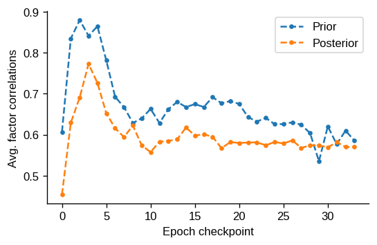
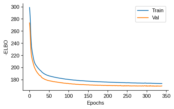
Epoch 338 train -ELBO: 173.508; val -ELBO: 169.339; val R2: 0.758; q(z) corr: 0.57; p(z) corr: 0.585:  68%|██████▊   | 339/500 [05:03<02:24,  1.12it/s]
/home/yinuo/Desktop/azizi_lab/IMS/models/base_model.py:490: UserWarning: FigureCanvasAgg is non-interactive, and thus cannot be shown
  fig.show()
/home/yinuo/Desktop/azizi_lab/IMS/models/base_model.py:470: UserWarning: FigureCanvasAgg is non-interactive, and thus cannot be shown
  fig.show()
/home/yinuo/Desktop/azizi_lab/IMS/env/lib/python3.9/site-packages/anndata/_core/aligned_df.py:68: ImplicitModificationWarning: Transforming to str index.
  warnings.warn("Transforming to str index.", ImplicitModificationWarning)

# Save results into a full h5ad (AnnData) carrying the latent embedding, the
# cell-interaction tensor, and cell-type labels.
results_dir = "../../results/"
if not os.path.exists(results_dir):
    os.makedirs(results_dir, exist_ok=True)
adata_xenium.write_h5ad(os.path.join(results_dir, "LYNX_breast_xenium.h5ad"))

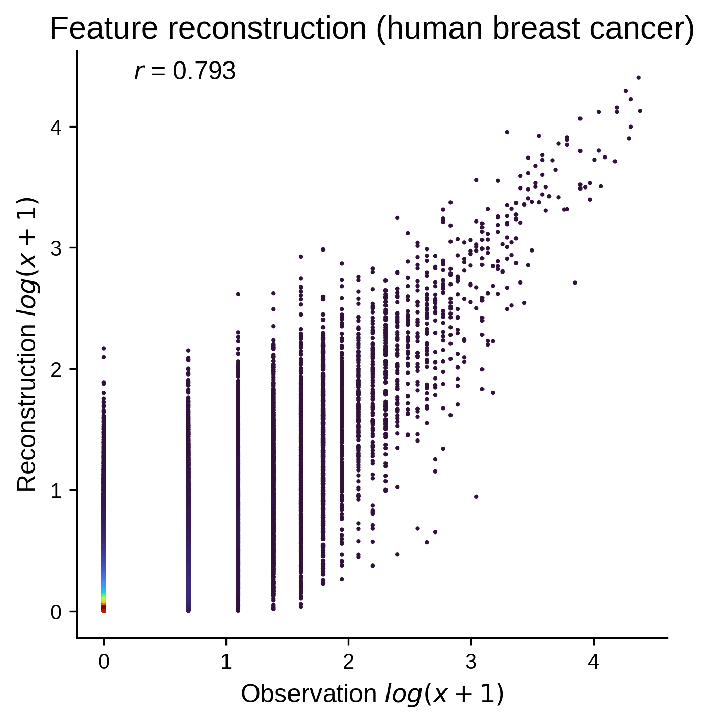
Reconstruction quality¶

Observed vs. reconstructed gene expression should fall along the diagonal.

[5]:

lynx.plot.disp_kde_scatter(
    adata_xenium.X.A.flatten().copy(),
    res.px.flatten().copy(),
    xlabel=r"Observation $log(x+1)$",
    ylabel=r"Reconstruction $log(x+1)$",
    title="Feature reconstruction (human breast cancer)",
)

4. Load the pre-saved result snapshot¶

Training above requires the full (large) Xenium / H&E inputs and a GPU. For the downstream analysis we load a LYNX result snapshot — the same object the training step produces, carrying the latent embedding X_z, the cell-type labels, and the inferred cell-interaction tensor (omega).

[6]:

results_dir = "../../results/"
adata = sc.read_h5ad(os.path.join(results_dir, "LYNX_breast_xenium.h5ad"))
adata.obs[cluster_key] = (
    adata_xenium.obs[cluster_key]
    .astype(str)
    .replace({"DCIS_1": "DCIS", "Prolif_Invasive_Tumor": "Invasive_Tumor"})
    .astype("category")
)

/home/yinuo/Desktop/azizi_lab/IMS/env/lib/python3.9/site-packages/anndata/_core/aligned_df.py:68: ImplicitModificationWarning: Transforming to str index.
  warnings.warn("Transforming to str index.", ImplicitModificationWarning)

5. Gradient Trajectory inference (principal tree)¶

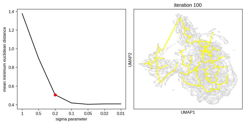
Fit a principal tree over the latent embedding. For hyperparameter choices, empirically ppt_lambda between [1e3, 1e4] gives a smooth, simplified manifold.

[7]:

principal_graph = lynx.trajectory.get_tree(
    adata,
    use_rep="X_z",
    n_nodes=int(0.01 * adata.n_obs),
    ppt_lambda=5e3,
    plot_graph=True,
)

fig, ax = plt.subplots(figsize=(6, 5), dpi=150)
scf.pl.graph(adata, basis="pca", ax=ax, title="Principal graph")

2026-06-24 23:38:15.396118: I tensorflow/core/platform/cpu_feature_guard.cc:210] This TensorFlow binary is optimized to use available CPU instructions in performance-critical operations.
To enable the following instructions: AVX2 FMA, in other operations, rebuild TensorFlow with the appropriate compiler flags.
2026-06-24 23:38:15.884775: W tensorflow/compiler/tf2tensorrt/utils/py_utils.cc:38] TF-TRT Warning: Could not find TensorRT

inferring a principal tree --> parameters used
    160 principal points, sigma = 0.2, lambda = 5000.0, metric = euclidean
    fitting:  19%|█▉        | 19/100 [00:01<00:05, 14.81it/s]
    converged
    finished (0:00:01) --> added
    .uns['ppt'], dictionnary containing inferred tree.
    .obsm['X_R'] soft assignment of cells to principal points.
    .uns['graph']['B'] adjacency matrix of the principal points.
    .uns['graph']['F'] coordinates of principal points in representation space.
    graph cleaned --> removed 14 principal points

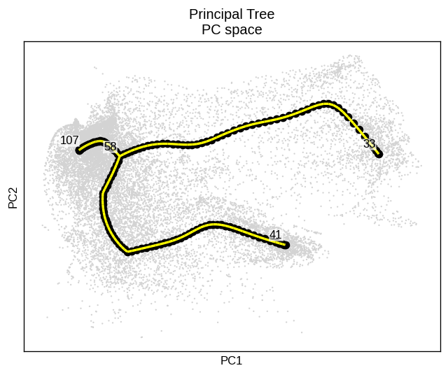
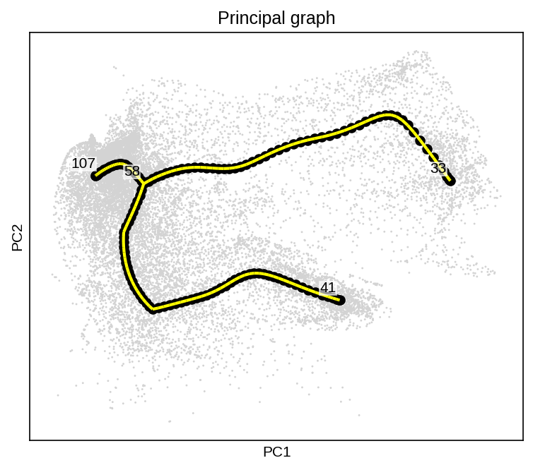
From the principal-tree visualization we pick the root, the branching node, and the two leaves, then compute pseudotime from the root.

[8]:

# Assign nodes based on visualized principal graph manifold
root_node = 107
branch_node = 58
leave_nodes = [33, 41]

# Mute FutureWarning from external scFates package
import warnings
with warnings.catch_warnings():
    warnings.simplefilter("ignore", FutureWarning)
    lynx.trajectory.compute_pseudotime(adata, principal_graph, source=root_node)

Computing pseudotime on principal tree...
node 107 selected as a root --> added
    .uns['graph']['root'] selected root.
    .uns['graph']['pp_info'] for each PP, its distance vs root and segment assignment.
    .uns['graph']['pp_seg'] segments network information.
projecting cells onto the principal graph
    finished (0:00:06) --> added
    .obs['edge'] assigned edge.
    .obs['t'] pseudotime value.
    .obs['seg'] segment of the tree assigned.
    .obs['milestones'] milestone assigned.
    .uns['pseudotime_list'] list of cell projection from all mappings.

6. Spatial visualizations¶

[9]:

# Inferred spatial gradient (pseudotime) in tissue coordinates
fig, ax = plt.subplots(dpi=150)
sq.pl.spatial_scatter(
    adata, color="t", cmap="RdBu_r",
    size=20, img=False, edgecolor="none",
    ax=ax, return_ax=True, title="Inferred spatial gradient",
)
plt.show()

# Spatial cell-type map
fig, ax = plt.subplots(dpi=150)
sq.pl.spatial_scatter(
    adata, color=cluster_key,
    img=False, size=15, ax=ax, return_ax=True, title="",
)
plt.show()

/home/yinuo/Desktop/azizi_lab/IMS/env/lib/python3.9/site-packages/squidpy/pl/_spatial_utils.py:488: FutureWarning: The default value of 'ignore' for the `na_action` parameter in pandas.Categorical.map is deprecated and will be changed to 'None' in a future version. Please set na_action to the desired value to avoid seeing this warning
  color_vector = color_source_vector.map(color_map)

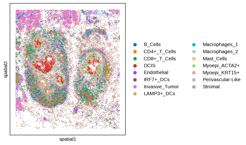
7. Cell-type composition dynamics¶

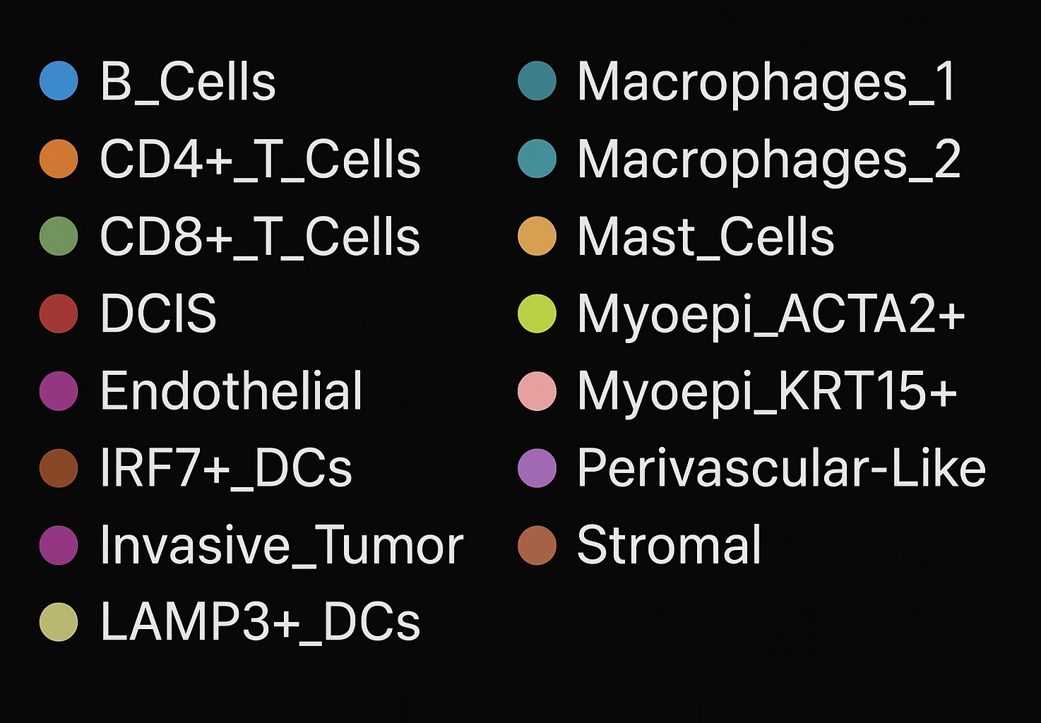
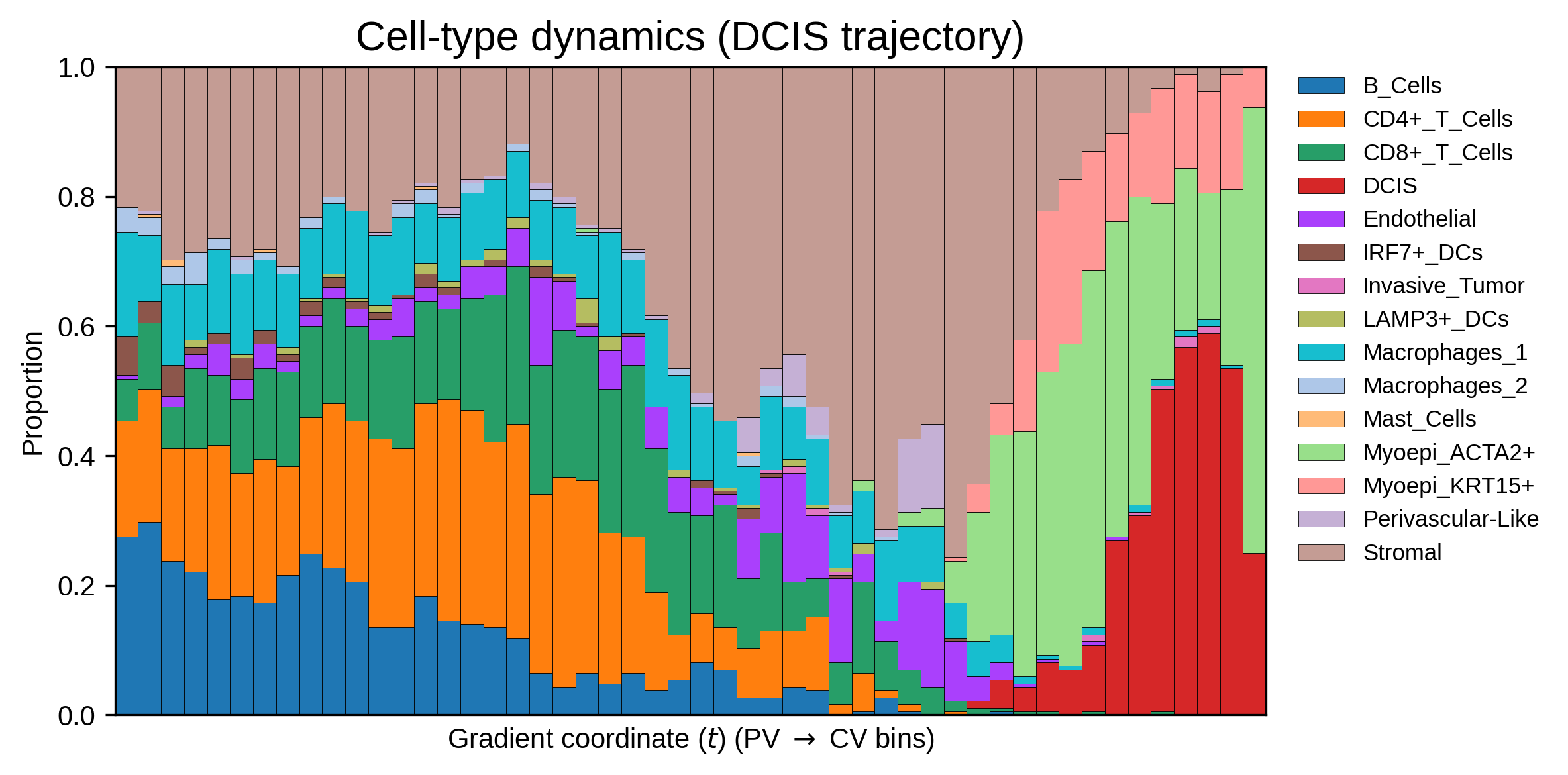
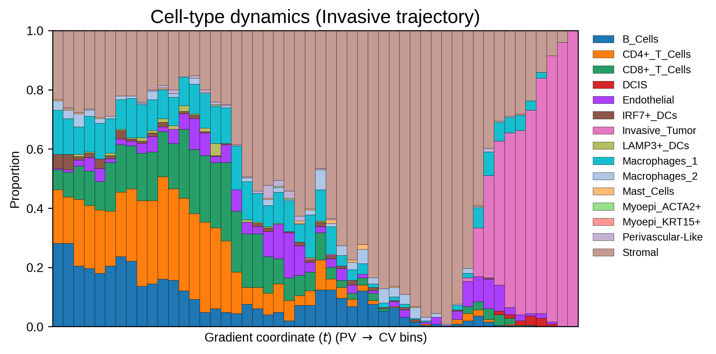
The spatial manifold from the inferred latent space shows a tree structure. In fact, coloring with cell-type labels shows a clear polarized phenotype change, particularly with distinct stromal environments towards DCIS & Invasive tumor states respectively:

Spatial \(\rightarrow\) PCA (gradient coordinate)	Spatial \(\rightarrow\) PCA (cell-type)	Cell-type labels

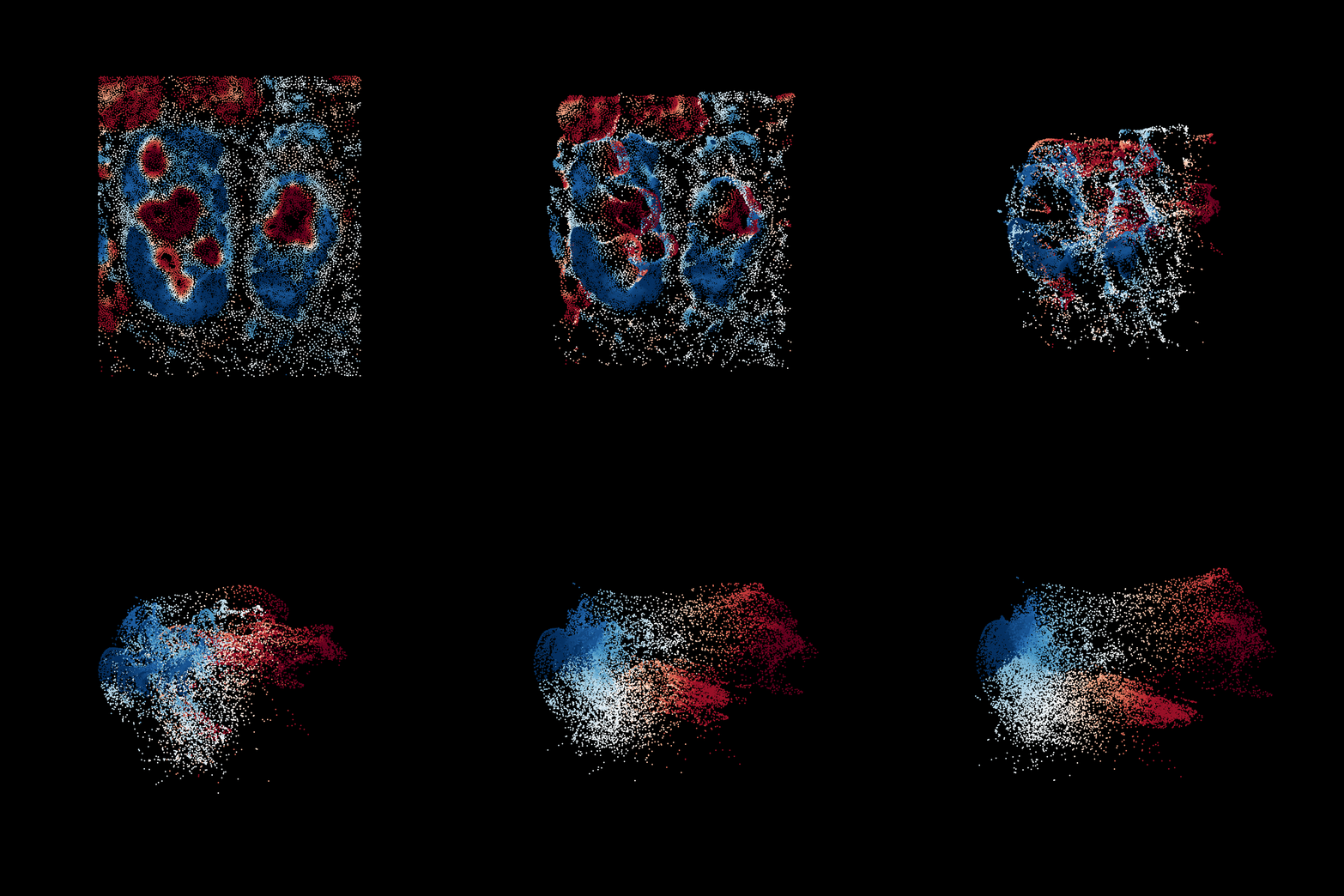
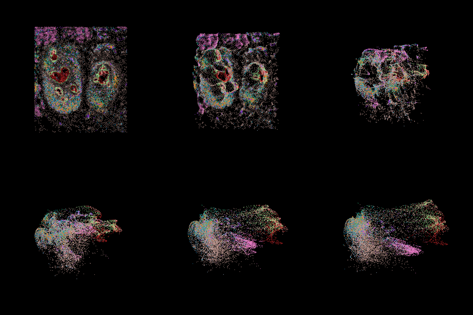
We can then split the tree into the immune→DCIS and immune→invasive paths, then show how cell-type composition shifts along each as a stacked dynamics plot. See this analysis script for detailed signature and pathway analyses.

[10]:

# Assign tree segments (immune root / DCIS branch / invasive branch).
root_path = lynx.trajectory.sort_nodes(adata, root_node=root_node, term_node=branch_node)
dcis_path = lynx.trajectory.sort_nodes(adata, root_node=branch_node, term_node=leave_nodes[0])[1:]
invasive_path = lynx.trajectory.sort_nodes(adata, root_node=branch_node, term_node=leave_nodes[1])[1:]

principal_assignments = adata.obsm["X_R"].argmax(1)
segments = []
for assign in principal_assignments:
    if assign in root_path:
        segments.append("immune")
    elif assign in dcis_path:
        segments.append("dcis")
    else:
        segments.append("invasive")
adata.obs["zone"] = segments

adata_norm = adata.copy()
sc.pp.normalize_total(adata_norm, target_sum=1e4)
sc.pp.log1p(adata_norm)

n_bins = 50
adata_dcis = adata_norm[adata_norm.obs["zone"].isin(["immune", "dcis"])].copy()
adata_dcis.obs_names = adata_dcis.obs_names.astype(str)
dcis_dynamic_df = lynx.utils.get_celltype_dynamics(
    adata_dcis, adata_dcis.obs[cluster_key], n_bins=n_bins
)

adata_invasive = adata_norm[adata_norm.obs["zone"].isin(["immune", "invasive"])].copy()
adata_invasive.obs_names = adata_invasive.obs_names.astype(str)
invasive_dynamic_df = lynx.utils.get_celltype_dynamics(
    adata_invasive, adata_invasive.obs[cluster_key], n_bins=n_bins
)

[11]:

fig, ax = lynx.plot.disp_stacked_dynamics(
    dcis_dynamic_df,
    colors=adata.uns["cell_type_colors"],
    title="Cell-type dynamics (DCIS trajectory)",
)
fig, ax = lynx.plot.disp_stacked_dynamics(
    invasive_dynamic_df,
    colors=adata.uns["cell_type_colors"],
    title="Cell-type dynamics (Invasive trajectory)",
)

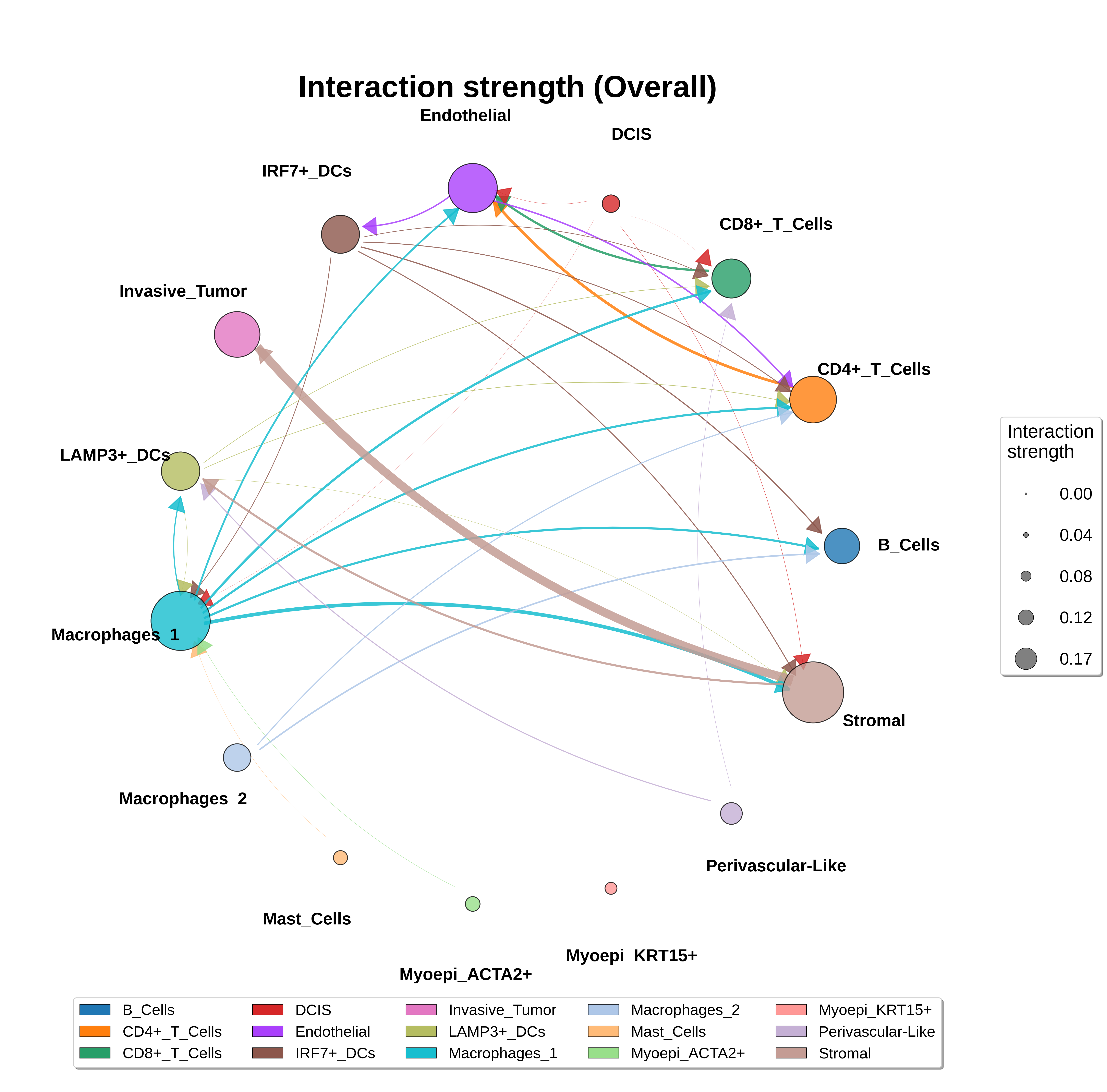
8. Example of cell–cell interactions summary¶

[12]:

cluster_labels = adata.obs[cluster_key].cat.categories
cci_df = lynx.plot.summarize_cell_interaction(
    adata, cluster_key=cluster_key,
    title="Interaction strength (Overall)", show_plot=False,
)
cci_df, pval_df = lynx.test_assoc.test_cci(adata, cci_df, cluster_labels, cluster_key=cluster_key)

fig, ax = lynx.plot.netVisual_circle(
    cci_df, figsize=(18, 18), min_threshold=0.0,
    colors=adata.uns["cell_type_colors"],
    title="Interaction strength (Overall)",
)